Quantum Mechanics 1

Fact

Einstein found that for any photon we have the relation

E = h ν

Superposition, Entanglement and Interaction Free Measurements

Definition

Spin is fundamental property of elementary particles dictating their internal(intrinsic) angular momentum

Example

linear superposition of spins

| Ψ ⟩ = | ↑, z ⟩ + | ↓, z ⟩

Example

tensor product states

(α_{1} | u_{1} ⟩ + α_{2} | u_{2} ⟩) \otimes (β_{1} | b_{1} ⟩ + β_{2} | v_{2} ⟩)

= α_{1} β_{1} | u_{1} ⟩ \otimes | v_{1} ⟩ + α_{1} β_{2} | u_{1} ⟩ \otimes | v_{2} ⟩ + α_{2} β_{1} | u_{2} ⟩ \otimes | v_{1} ⟩ + α_{2} β_{2} | u_{2} ⟩ \otimes | v_{2} ⟩

but nice we cant have

| u_{1} ⟩ \otimes | v_{1} ⟩ + | u_{2} ⟩ \otimes | v_{2} ⟩

as that will imply

$α_{1} β_{1} = α_{2} β_{2} = 1$ and $α_{1} β_{2} = α_{2} β_{1} = 0$ which is a contradiction a s that would mean $α_{1} β_{1}$ and $α_{2} β_{2}$ is either 1 or 0. So we have an unfactorizable/entangled

Photoelectric effect

Fact

Key findings from photoelectric effect experiments:

critical frequency $ν_{0}$ above which a current is measured but below nothing happens
light thought of as quantized bundles of energy(photon) with $E = h ν$ where h is the planck constant

Definition

For any surface work function(W) is the energy needed to release an electron to the vacuum around the surface

Definition

the compton wavelength of a particle of mass m is $λ c = \frac{h}{m c}$

Proposition

De Broglie(1924) stated that:
The wave partice duality is universal for all matter for each particle of momentum $ρ$ we have an associated plane wave of wavelength $λ_{p} = \frac{h}{ρ}$ known as the de Broglie wavelength

de Broglie Waves, Propagation and the Free Particle

we may rexpress de Broglie's relation as

p = \frac{h}{λ} = \frac{h}{2 π} \frac{2 π}{λ} = \bar{h} k

where $\bar{h}$ is the reduced planck's constant and $k$ is the wave number

something unusual arises.

Proposition

De Broglie wavelengths are not galliean invariant!

Proof.
First we recall in a galilean transformation we have

x^{'} = x - v t and t^{'} = t

so to find the relations for velocity and momentum we take the derivative to see that

\frac{d x^{'}}{d t^{'}} = \frac{d x}{d t} - v

so that we have ${\tilde{v}}^{'} = \tilde{v} - v$ for ${\tilde{v}}^{'}$ observed in the $S^{'}$ frame. With this we obtain

p^{'} = p - m v \to λ = \frac{h}{p^{'}} = \frac{h}{p - m v} \neq λ

$◻$

This is in stark contrast with ordinary waves. To see this we use the relation for phase $k x - w t$ where $k = \frac{2 π}{λ}$ is the wave number. Then

ϕ = k (x - \frac{ω}{k} t) = \frac{2 π}{λ} (x - V t) = \frac{2 π x}{λ} - \frac{2 π V}{λ} t .

where we use the fact that $\frac{ω}{k} = \frac{2 π f}{2 π / λ} = λ f = V$ is the speed of the wave (not the same as the observer's relative velocity v). Since this quantity is Galilean invariant, observers at S and S' should see the same phase for the same point at the same time, meaning that

ϕ = \frac{2 π}{λ} (x - v t) = \frac{2 π}{λ} (x^{'} + v t - V t) = \frac{2 π}{λ} x^{'} - (V - v) t^{'},

which further simplifies to

= \frac{2 π}{λ} x^{'} - \frac{2 π}{λ} V (1 - \frac{v}{V}) t^{'},

should be equal to the phase $ϕ^{'} = \frac{2 π}{λ} x^{'} - \frac{2 π V}{λ} t^{'}$ seen by the moving observer. In particular, the wavenumber and
angular frequency satisfy $k^{'} = \frac{2 π}{λ}$ and $ω^{'} = \frac{2 π}{λ} V (1 - \frac{v}{V})$ , so that

ω^{'} = ω (1 - \frac{v}{V}), k^{'} = k ⟹ λ^{'} = λ

Question

So what is the implication of the wavelength of matter waves changing under gallilean transformations?

First assume the wavefuction form $e^{i (k x - ω t)}$ which you will learn later. Then you simply sub in the relations we found above. To do so for convenience we choose to write the phase in terms of the momentum and energy of the wave:

\frac{1}{h} ϕ = ℏ k x - ℏ ω t = p x - \frac{p^{2}}{2 m} t

Where momentum undergoes the transformation

p^{'} = p - m v

Thus, this must be equal to:

\frac{1}{h} ϕ = (p^{'} + m v) (x^{'} + v t) - \frac{(p^{'} + m v)^{2}}{2 m} t

= p^{'} x + p^{'} σ t + m v x^{'} + m v^{2} t - \frac{p^{' 2}}{2 m} t - p^{'} σ t - \frac{1}{2} m v^{2} t

= p^{'} x + m v (x - v t) - \frac{p^{' 2}}{2 m} t + \frac{1}{2} m v^{2} t

= p^{'} x + m v x - m v^{2} t - E^{'} t + \frac{1}{2} m v^{2} t

= p^{'} x - E^{'} t + m v x - \frac{1}{2} m v^{2} t

The first two terms are the phase of the primed wavefunction. The last two terms gives rise to $f (x, t)$ to be:

f (x, t) = \exp (\frac{i}{ℏ} (m v x - \frac{1}{2} m v^{2} t))

Proposition

Second de Broglie Relation:
Previously we had $p = \bar{h} k$ we find that we also have $E = \bar{h} ω$

Phase and group velocities

Definition

The group velocity of a wave with phase $k x - ω t$ is

v_{group} = \frac{d ω}{d k} |_{k}

evaluated at the wavenumber k that we're propagating.

In general the group velocity represents the velocity of a wave packet constructed under superpsotiions

So we then consider a superposition of plane waves $e^{i (k x - w (t) t)}$ by

Ψ (x, t) = \int d k Φ (k) e^{i (k x - ω (k) t)}

where $Ψ (x, t)$ is the wave packet(plane waves collectively considered together as a packet) defined at position and time

$e^{i (k x - ω (k) t)}$ represents a wave of wavenumber k and angular frequency $ω (k)$ and $Φ (k)$ is the ampltidude of the wave and this wave number $k$ . Now suppose that $Φ (k)$ is peaked at $k = k_{0}$ .

now write $ω$ as a taylor expansion

ω (k) = ω (k_{0}) + (k - k_{0}) {\frac{d ω}{d k} |}_{k = k_{0}} + O ((k - k_{0})^{2}),

because the value of $k$ that matter must be very close to $k_{0}$ given that $Φ (k)$ peaks there

Ψ (x, t) = \int d κ Φ (k) e^{i k x} e^{- i ω (k_{0}) t} e^{- i k \frac{d ω}{d k} |_{k_{0}} t} e^{i k_{0} \frac{d ω}{d k} |_{k_{0}} t} e^{(negligible)}

= e^{- i ω (k_{0}) t} e^{i k_{0} \frac{d ω}{d k} |_{k_{0}} t} \int d k Φ (k) e^{i k x} e^{- i k \frac{d ω}{d k} |_{k_{0}} t} .

taking the magnitude on both sides we get

| Ψ (x, t) | = | Ψ (x - {\frac{d ω}{d k} |}_{k_{0}} t, 0) | .

this shows that indeed the shape of the wave packet moves at the group velocity

In fact this taylor expansion justifies what is known as the principal of stationary phase which is based on the intuitition that say for an expression like $\int f (x) \sin x$ which is positive half the time and negative the half the time so it will contribute very little if $f$ is slowly varying relative to $\sin x$

Specifically in our case taking the phase $ϕ (k) = k x - ω (k) t$ interpret slowly varying/stationary phase by

0 = {\frac{d ϕ (k)}{d k} |}_{k_{0}} = x - {\frac{d ω (k)}{d k} |}_{k_{0}} t = 0,

where we get $x = \frac{d ω}{d k} |_{k_{0}} t$ which also shows the group velocity is indeed the speed at which the wave packet is propagating.

5. Wavefunction

To get a general form for a wavefunction we first choose from 4 potential periodic functions expressed in terms of phase $k x - ω t$

$\sin (k x - ω t)$
$\cos (k x - ω t)$
$e^{i (k x, ω t)} = e^{i k x} e^{- i ω t}$
$e^{- i (k x - ω t)} = e^{- i k x} e^{i ω t}$

The wave function represents the probability of particle as position at a certain time. Hence at any time, the total the wave function cannot be all zero as that will mean the all the entire wave "vanished"

However for 1 and 2 clearly a certain periodic time intervals they will disappear. For example for (1)

Ψ (x, t) = \sin (k x - ω t) + \sin (k x + ω t)

as there is an equal probaility of the particle found moving in the $+ x$ and $- x$ directions but upon expanding this we get

Ψ (x, t) = 2 \sin (k x) \cos (ω t)

which is zero when $ω t = (\frac{π}{2}, \frac{3 π}{2}, \frac{5 π}{2} \dots)$ . In contrast for 3,4 take for example 3 we have again

Ψ = e^{i (k x - ω t)} + e^{i (- k x - ω t)} = 2 \cos k x e^{i ω t}

which is again because there is an equal probability of moving $+ x$ and $- x$ but here it is never zero any time for all values of x. Using a similar process we obtain $2 \cos k x e^{- i ω t}$

Question

Therefore because both 3 and 4 are valid solutions we superimpose in them to get the full solution?

Nope we cant

Ψ (x, t) = e^{i (k x - ω t)} + e^{- i (k x - ω t)} = 2 \cos (k x - ω t)

but this is the form of (2) which we have proven above is not valid! So we must choose between (3) and (4). The choice happens to be a matter of convnetion which is defined to be

Ψ (x, t) = e^{i (k x - ω t)}

to be the free particle wave function where $p = \bar{h} k, E = \bar{h} ω, E = \frac{p^{2}}{2 m}$ if you recall

We now want to find an operator that can extract information from the wave function, something like a derivative. More precisely notice that

\frac{\bar{h}}{i} \frac{\partial}{\partial x} Ψ (x, t) = \frac{\bar{h}}{i} (i k) Ψ (x, t) = \bar{h} k Ψ (x, t) = p Ψ (x, t)

so it makes sense to identify this with what is known as the momentum operator $\hat{p}$

Definition

momentum operator is defined by

\hat{p} \equiv \frac{\bar{h}}{i} \frac{\partial}{\partial x}

and so we have

\hat{p} Ψ = p Ψ

this looks quite similar to linear algebra. Remember eigenvalues where we have $A x = λ x$ we have a similar form here. With this inspiration the function $Ψ (x, t)$ is called an eigenstate of the operator $\hat{p}$ with eigenvalue p.

Now that we have extracted the momentum it makes sense that we also want to extract information regarding the energy of the wave function. Now instead of taking the spatial derivative lets see what happens when we take the time derivative instead so now we obtain

i \hat{h} \frac{\partial}{\partial t} Ψ = (i \hat{h}) (- i ω) Ψ = \hat{h} ω Ψ = E Ψ

since $Ψ = e^{i k x} e^{- i ω t}$ . This results in yet another eigenvalue equation

It turns out we can extract more physics by combining this with our previous relation for momentum. In particular because $E = \frac{p^{2}}{2 m}$ and $p Ψ = \hat{p} Ψ$ we have

E Ψ = \frac{p}{2 m} (p Ψ) = \frac{p}{2 m} \frac{\hat{h}}{i} \frac{\partial}{\partial x} Ψ

where we have simply replace $(p Ψ)$ with the momentum operator. But because the p term in the $\frac{p}{2 m}$ fraction outside is also a constant(relative to x) we can move it in like so to obtain

\frac{1}{2 m} \frac{\hat{h}}{i} \frac{\partial}{\partial x} (p Ψ) = \frac{1}{2 m} \frac{\hat{h}}{i} \frac{\partial}{\partial x} (\frac{\hat{h}}{i} \frac{\partial}{\partial x} Ψ) = \frac{- {\hat{h}}^{2}}{2 m} \frac{\partial^{2}}{\partial x^{2}} Ψ

this then motivates the following definition

Definition

energy operator:

\hat{E} = - \frac{{\bar{h}}^{2}}{2 m} \frac{\partial^{2}}{\partial x^{2}}

so combining this with above we can see that

- \frac{{\bar{h}}^{2}}{2 m} \frac{\partial^{2}}{\partial x^{2}} Ψ = i \bar{h} \frac{\partial}{\partial t} Ψ

this is known as the free schrodinger equation. Looking at the energy operator $\hat{E} = \frac{{\hat{p}}^{2}}{2 m}$ it looks like our usual "kinetic energy" in classical mechanics. The next natural step is to then add in a potential $V (x, t)$ so that our total energy is $E = \frac{p^{2}}{2 m} + V$ . So we then modify our energy operator expression using by defining

Definition

Hamiltonian operator

\hat{H} = \frac{{\hat{p}}^{2}}{2 m} + V (x, t)

this then allows us to write the general Schrodinger equation

Theorem

1-D Schrodinger Equation:
The the wave function $Ψ$ in one dimension satisfies $i \bar{h} \frac{\partial}{\partial t} Ψ = \hat{H} Ψ$

i \bar{h} \frac{\partial Ψ}{\partial t} = (- \frac{{\bar{h}}^{2}}{2 m} \frac{\partial^{2}}{\partial t^{2}} + V (x, t)) Ψ

Definition

The position operator denoted by $\hat{x}$ multiplies functions by $x$

\hat{x} f (x) = x f (x)

Lets try to investigate the properties of these operators, in particular whether they commute.

Example

We determine whether $\hat{x}$ and $\hat{p}$ commuate by computing the difference between $\hat{x} \hat{p} ϕ$ and $\hat{p} \hat{x} ϕ$ for some function $ϕ (x, t)$

\hat{x} (\hat{p} ϕ) - \hat{p} (\hat{x} ϕ) = \hat{x} (\frac{\bar{h}}{i} \frac{\partial}{\partial x} ϕ) - \hat{p} (x ϕ) = \frac{\bar{h}}{i} x \frac{\partial}{\partial x} ϕ - \frac{\bar{h}}{i} \frac{\partial}{\partial x} (x ϕ)

now using product rule on the second term we see that

= \frac{\bar{h}}{i} x \frac{\partial}{\partial x} ϕ - \frac{\bar{h}}{i} ϕ - \frac{\bar{h}}{i} x \frac{\partial}{\partial x} ϕ = i \bar{h} ϕ

therefore we realized that they don't commute and writing the operators on one side and the operand on the other we have

(\hat{x} \hat{p} - \hat{p} \hat{x}) ϕ = i \bar{h} ϕ

Definition

The commutator of two operators $\hat{A}$ and $\hat{B}$ is denoted by $[\hat{A}, \hat{B}]$ refers to the operator $\hat{A} \hat{B} - \hat{B} \hat{A}$

Proposition

We have the equality of operators

[\hat{x}, \hat{p}] = \hat{x} \hat{p} - \hat{p} \hat{x} = i \bar{h}

recall that we have our expression for the 1D schrodinger equation from earlier. Can we generalize this to 3D? That is

Theorem

3D Schrodinger Equation:

i \bar{h} \frac{\partial Ψ}{\partial t} = (- \frac{{\bar{h}}^{2}}{2 m} \nabla^{2} + V (\vec{x}, t)) Ψ

we will be dealing with it more in detail when we solve differential equations later but as a preview it is to be noted that we now have

[{\hat{x}}_{i}, {\hat{p}}_{j}] = i \bar{h} δ_{i j}

Probability Density, Current and Conservation

Now recall that the wave function is a probability function of a particle at $(x, t)$ and returns a complex number. Therefore we must have

1 = \int_{\infty}^{\infty} | Ψ (x, t)^{2} | d x

First we assume some boundary conditions in particular

lim_{x \to \pm \infty} Ψ (x, t) = 0

Remark

While there are technically mathematical examples where $Ψ (x, t)$ does not have a limit as $x \to \infty$ and the integrral of $| Ψ |^{2}$ still converges those examples do not pop up in physical contexts and thus we are (mostly) safe to ignore them

in addition we require that the function $Ψ$ does not oscillate too quickly in particular

\frac{\partial Ψ (x, t)}{\partial x} is bounded as x \to \pm \infty

Essentially we need some "regularity"

Definition

For a wave function $Ψ (x, t)$ with $\int_{- \infty}^{\infty} | Ψ (x, t) |^{2} d x$ equal to some finite number $N$ we say that $Ψ$ is normalizable and we let $Ψ^{'} = \frac{Ψ}{\sqrt{N}}$ be the associated normalized wavefunction

That is

\int_{- \infty}^{\infty} | Φ^{'} (x, t) |^{2} d x = \int_{- \infty}^{\infty} \frac{| Ψ (x, t) |^{2}}{N} d x = \frac{N}{N} = 1

So now want to check of the conversation of probability is satisfied that is

\int Ψ^{*} (x, t_{0}) Ψ (x, t_{0}) d x = 1

Here we let $Ψ^{*} (x, t_{0}) Ψ (x, t_{0})$ be called the probability density and denote it by $ρ (x, t)$ . Then we define $N (t) = \int ρ (x, t) d x$ and we then wish to show that $N (t) = 1$ for all $t > t_{0}$ given that $N (t_{0}) = 1$

We can show this by showing $\frac{d N}{d t} = 0$ so

\frac{d N}{d t} = \int \frac{\partial}{\partial t} ρ (x, t) d x = \int (\frac{\partial Ψ^{*}}{\partial t} Ψ + Ψ^{*} \frac{\partial Ψ}{\partial t}) d x

where we basically differentiated under integral since bounded. Then using the relation from Schrodinger equation

i \bar{h} = \hat{H} \leftrightarrow \frac{\partial Ψ}{\partial t} = - \frac{i}{\bar{h}} \hat{H} Ψ

But we also have a time deritive of the complex conjugate above so

- i \bar{h} {(\frac{\partial Ψ}{\partial t})}^{*} = (\hat{H} Ψ)^{*} \leftrightarrow \frac{\partial Ψ^{*}}{\partial t} = - \frac{i}{\bar{h}} (\hat{H} Ψ)^{*}

because the complex conjugate of the partial derivative is also the the partial derivative of the complex conjugate. Plugging these back we get

\frac{d N}{d t} = \int \frac{i}{\bar{h}} ((\hat{H} Ψ)^{*} ψ - Ψ^{*} (\hat{H} Ψ)) d x

and in order for this to be zero we essentially require

\int (\hat{H} Ψ)^{*} Ψ d x = \int Ψ^{*} (\hat{H} Ψ) d x

to hold. This motivates the following definition

Definition

For any (linerar) opreator $T$ the Hermitian conjugate of $T$ denoted by $T^{*}$ or $T^{†}$ is the linear operator that satisfies

\int Ψ_{1}^{*} T Ψ_{2} = \int (T^{†} Ψ_{1})^{*} Ψ_{2}

we say that $T$ is Hermitian if $T = T^{*}$

We now plug in the from the definition of $\hat{H} = - \frac{{\bar{h}}^{2}}{2 m} \frac{\partial^{2}}{\partial x^{2}} + V (x, t)$ to get

\frac{d N}{d t} = \int \frac{i}{ℏ} ((\hat{H} Ψ)^{\*} Ψ - Ψ^{\*} (\hat{H} Ψ)) d x = \int \frac{i}{ℏ} ((\hat{H} Ψ)^{\*} Ψ - Ψ^{\*} (\hat{H} Ψ)) d x

= \int \frac{i}{ℏ} (- \frac{ℏ^{2}}{2 m} \frac{\partial^{2} Ψ^{\*}}{\partial x^{2}} Ψ + V (x, t) Ψ^{\*} Ψ + \frac{ℏ^{2}}{2 m} Ψ^{\*} \frac{\partial^{2} Ψ}{\partial x^{2}} - Ψ^{\*} V (x, t) Ψ) d x,

We have used the fact that $V (x, t)$ is always real(because it is some energy). Therefore these terms cancel out and we are left with

= - \frac{i ℏ}{2 m} \int (\frac{\partial^{2} Ψ^{\*}}{\partial x^{2}} Ψ - Ψ^{\*} \frac{\partial^{2} Ψ}{\partial x^{2}}) d x .

A common way in physics to show an integral vanishes is by showing that is a total deriviatve

\frac{\partial^{2} Ψ^{\*}}{\partial x^{2}} Ψ - Ψ^{\*} \frac{\partial^{2} Ψ}{\partial x^{2}} = \frac{\partial}{\partial x} (\frac{\partial Ψ^{\*}}{\partial x} Ψ - Ψ^{\*} \frac{\partial Ψ}{\partial x})

plugging this back in we get

\frac{d N}{d t} = \int - \frac{\partial}{\partial x} [\frac{ℏ}{2 i m} (Ψ^{\*} \frac{\partial Ψ}{\partial x} - Ψ \frac{\partial Ψ^{\*}}{\partial x})] d x = {[\frac{\bar{h}}{2 i m} (Ψ^{*} \frac{\partial Ψ}{\partial x} - Ψ \frac{\partial Ψ^{*}}{\partial x})]}_{- \infty}^{\infty} = 0

because remember that $\frac{\partial Ψ}{\partial x}$ and $\frac{\partial Ψ^{*}}{\partial x}$ is bounded from our boundary conditions. Therefore our definition for the wave function is indeed normalizable

However we also notice inside the brackets we have the form $z - z^{*} = 2 i Im (z)$ so therefore we may rewrite this as

\frac{\partial ρ}{\partial t} = - \frac{\partial}{\partial x} [\frac{ℏ}{m} Im (Ψ^{\*} \frac{\partial Ψ}{\partial x})] .

Definition

The current density $J (x, t)$ for the wavefunction $Ψ (x, t)$ is given by

J (x, t) = \frac{\bar{h}}{m} Im (Ψ^{*} \frac{\partial Ψ}{\partial x})

and we so may rewrite our above calculations in the simpler form

\frac{\partial p}{\partial t} = - \frac{\partial J}{\partial x} \to \frac{\partial p}{\partial t} + \frac{\partial J}{\partial x} = 0

which is a current conservation statement similar to what we might have seen in electromagnetism.

Fourier Transforms, Uncertainty and Time Evolution

We begin today by discussing wave packets and uncertainty.

Consider a wave function of the form

Ψ (x, 0) = \frac{1}{\sqrt{2} π} \int ϕ (k) e^{i k x} d k

this is essentially a superposition of plane waves( $e^{i k x}$ ) of different wavelengths. Just see that the integral is simply a continuous sum

Theorem

Fourier Inversion:
Suppose $Ψ (x, 0) = \frac{1}{\sqrt{2} π} \int ϕ (k) e^{i k x} d k$ we can recover coefficients via fourier inversion

ϕ (k) = \frac{1}{\sqrt{2} π} \int Ψ (x, 0) e^{- i k x} d x

we briefly touched on this in our earlier discussions on group velocity but not we focus on how to understand uncertainties of position and momentum through this result

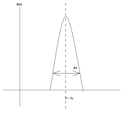
first consider $Φ (k)$ symmetric and centered about $k = k_{0}$ with width $Δ k$

attachments/Quantum Mechanics 1 2025-06-12 16.37.34.excalidraw.png

Proposition

$Ψ (x, 0)$ is real if and only if $Φ^{*} (- k) = Φ (k)$ is real

Proof.
Begin by complex conjugating the expression (1.1) for $Ψ (x, 0)$ :

Ψ^{\*} (x, 0) = \frac{1}{\sqrt{2 π}} \int_{- \infty}^{\infty} Φ^{\*} (k) e^{- i k x} d k = \frac{1}{\sqrt{2 π}} \int_{- \infty}^{\infty} Φ^{\*} (- k) e^{i k x} d k .

In the second step we let $k \to - k$ in the integral, which is allowable because we are integrating over

all k, and the two sign flips, one from the measure dk and one from switching the limits of integration,

cancel each other out. If $Φ^{\*} (- k) = Φ (k)$ then

Ψ^{\*} (x, 0) = \frac{1}{\sqrt{2 π}} \int_{- \infty}^{\infty} Φ (k) e^{i k x} d k = Ψ (x, 0),

as we wanted to check. If, on the other hand we know that $Ψ (x, 0)$ is real then the equality of $Ψ^{\*}$ and

$Ψ$ gives

\frac{1}{\sqrt{2 π}} \int_{- \infty}^{\infty} Φ^{\*} (- k) e^{i k x} d k = \frac{1}{\sqrt{2 π}} \int_{- \infty}^{\infty} Φ (k) e^{i k x} d k .

This is equivalent to

\frac{1}{\sqrt{2 π}} \int_{- \infty}^{\infty} (Φ^{\*} (- k) - Φ (k)) e^{i k x} d k = 0.

This equation actually means that the object over the brace must vanish. Indeed, the integral is

computing the Fourier transform of the object with the brace, and it tells us that it is zero. But a

function with zero Fourier transform must be zero itself (by the Fourier theorem). Therefore reality

$◻$

but the condition that $Ψ^{*} (- k) = Ψ (k)$ is not true in our case unless $k_{0} = 0$ (essentially we need $Ψ (k)$ to be symmetric about zero for this condition to be true)

Momentum Space and Expectation Values

Recalling that we have the fourier decompositions

Ψ (x) = \frac{1}{\sqrt{2 π}} \int Φ (k) e^{i k x} d k,

Φ (k) = \frac{1}{\sqrt{2 π}} \int Ψ (x) e^{- i k x} d k .

you might decide to combine both to get a single expression for the wave function like so

Ψ (x) = \frac{1}{\sqrt{2 π}} \int [\frac{1}{\sqrt{2 π}} \int Ψ (x^{'}) e^{- i k x^{'}} d x^{'}] e^{i k x} d k,

rearranging in this way we seemed to have isolated a perculiar "function"(spoiler it isn't a function)

Ψ (x) = \int_{- \infty}^{\infty} Ψ (x^{'}) \frac{1}{2 π} \int e^{i k (x - x^{'})} d k d x^{'} .

Definition

The Dirac delta function is a "function" given by

δ (x - x^{'}) = \frac{1}{2 π} \int_{- \infty}^{\infty} e^{i k (x - x^{'})} d k .

we have essentially demonstrated the sifting property of the dirac delta function that is

Ψ (x) = \int_{- \infty}^{\infty} Ψ (x^{'}) δ (x - x^{'}) d x^{'}

where

δ (x - x^{'}) = {\begin{cases} 1 & x = x^{'} \\ 0 & x \neq x^{'} \end{cases}

note that $δ$ isn't even a function. The cases the above is just an informal way of describing the effect of integrating $Ψ (x)$ with the dirac delta function $δ (x - x^{'})$ . You should refer to Differential Analysis to learn what exactly $δ$ is and why it isn't a function.

Recall that we prove our normalization condition by showing that

\int Ψ^{*} (x) Ψ (x) d x = 1

We now want to do the same for $Φ (x)$ .

First using different variables of integration k, k' for the two terms (but the same x):

\int Ψ^{\*} (x) Ψ (x) d x = \int (\frac{1}{\sqrt{2 π}} \int Φ^{\*} (k) e^{- i k x} d k) (\frac{1}{\sqrt{2 π}} \int Φ (k^{'}) e^{i k^{'} x} d k) d x .

From here, we know that we can't do the integrals over k in general, since those are in the most general form possible, and thus it makes sense to try to do the x-integral. Rewriting the order of the integrals, we have

= \int Φ^{\*} (k) \int Φ (k^{'}) (\frac{1}{2 π} \int e^{i (k^{'} - k) x} d x) d k^{'} d k,

and now the inner integral is indeed the delta function $δ (k^{'} - k)$ , just with different dummy variables, so this simplifies to

= \int Φ^{\*} (k) \int Φ (k^{'}) δ (k - k^{'}) d k^{'} d k = \int Φ^{\*} (k) Φ (k) d k .

Essentially we just proved the following

Theorem

Parseval-Plancheral Identity:
For any function $Ψ (x)$ with Fourier transform $Φ (k)$ , we have

\int | Ψ (x) |^{2} d x = \int | Φ (k) |^{2} d k .

Recalling that $Ψ (x, t)$ has a probabilistic interpretation and that $\int_{- \infty}^{\infty} Ψ (x, t)^{*} Ψ (x, t) d x = 1$ plancheral identity hints that $Φ (k)$ perhaps too as a probabilistic interpretation.

First recall from our discussions above regarding the momentum operator that we associate our plane waves( $e^{i k x}$ ) with eigenstates of momentum $\hat{p} Ψ (x, t) = p Ψ (x, t)$ . Knowing that $p = \bar{h} k$ let us attempt to write plancheral relation in terms of momentum instead of $k$ . In doing so we obtain

\begin{aligned} Ψ (x) & = \frac{1}{\sqrt{2 π} ℏ} \int_{- \infty}^{\infty} \tilde{Φ} (p) e^{i p x / ℏ} d p, \\ \tilde{Φ} (p) & = \frac{1}{\sqrt{2 π}} \int_{- \infty}^{\infty} Ψ (x) e^{- i p x / ℏ} d x . \end{aligned}

by performing change of variables $p = \bar{h} k$ and $\tilde{Φ} (p) = Φ (k)$ . We write this in a more symmetric form by letting $\tilde{Φ} (p) \to Φ (p) \sqrt{\bar{h}}$ to get

Ψ (x) = \frac{1}{\sqrt{2 π ℏ}} \int_{- \infty}^{\infty} Φ (p) e^{i p x / ℏ} d p,

Φ (p) = \frac{1}{\sqrt{2 π ℏ}} \int_{- \infty}^{\infty} Ψ (x) e^{- i p x / ℏ} d x .

\int_{- \infty}^{\infty} d x | Ψ (x) |^{2} = \int_{- \infty}^{\infty} d p | Φ (p) |^{2} .

with this we make the following proposition

Proposition

$| Φ (p)^{2} |$ is the probability to find the particle with momentum in the range $(p, p + d p)$

let us verify this by discussing the expectation values of operators which is one of the first steps towards a full interpretation of quantum mechanics.

Definition

Let Q be a random variable which can take values in a finite set ${Q_{1}, \dots, Q_{n}}$ with probabilities $p_{1}, \dots, p_{n}$ , respectively. Then Q has expectation or expected value

⟨ Q ⟩ = \sum_{i = 1}^{n} p_{i} Q_{i} .

so since we took $Φ^{*} Φ$ to be our probability density function(for particle to be found in $[x, x + d x]$ ) our expected value for x will then be

⟨ \hat{x} ⟩ \equiv \int_{- \infty}^{\infty} x Ψ^{\*} (x, t) Ψ (x, t) d x .

similarly for momentum we have the expectation of the momentum operator as

⟨ \hat{p} ⟩ \equiv \int_{- \infty}^{\infty} p Φ^{\*} (p, t) Φ (p, t) d p .

but what form does this exactly take? lets see

⟨ \hat{p} ⟩ = \int_{- \infty}^{\infty} p Φ^{\*} (p, t) Φ (p, t) d p

= \int_{- \infty}^{\infty} d p p \int_{- \infty}^{\infty} \frac{d x}{\sqrt{2 π ℏ}} e^{i p x / ℏ} Ψ^{\*} (x, t) \int_{- \infty}^{\infty} \frac{d x^{'}}{\sqrt{2 π ℏ}} e^{- i p x^{'} / ℏ} Ψ (x^{'}, t)

= \frac{1}{2 π ℏ} \int_{- \infty}^{\infty} d x Ψ^{\*} (x, t) \int_{- \infty}^{\infty} d x^{'} Ψ (x^{'}, t) \int_{- \infty}^{\infty} d p p e^{i p x / ℏ} e^{- i p x^{'} / ℏ}

= \frac{1}{2 π ℏ} \int_{- \infty}^{\infty} d x Ψ^{\*} (x, t) \int_{- \infty}^{\infty} d x^{'} Ψ (x^{'}, t) \int_{- \infty}^{\infty} d p (\frac{ℏ}{i} \frac{\partial}{\partial x}) e^{i p x / ℏ} e^{- i p x^{'} / ℏ}

= \int_{- \infty}^{\infty} d x Ψ^{\*} (x, t) \int_{- \infty}^{\infty} d x^{'} Ψ (x^{'}, t) (\frac{ℏ}{i} \frac{\partial}{\partial x}) \frac{1}{2 π ℏ} \int_{- \infty}^{\infty} d p e^{i p x / ℏ} e^{- i p x^{'} / ℏ} .

letting $p = \bar{h} u$ in the final integral we have

\frac{1}{2 π ℏ} \int_{- \infty}^{\infty} d p e^{i p x / ℏ} e^{- i p x^{'} / ℏ} = \frac{1}{2 π} \int_{- \infty}^{\infty} d u e^{i u (x - x^{'})} = δ (x - x^{'}) .

as a result

⟨ \hat{p} ⟩ = \int_{- \infty}^{\infty} d x Ψ^{\*} (x, t) \int_{- \infty}^{\infty} d x^{'} Ψ (x^{'}, t) (\frac{ℏ}{i} \frac{\partial}{\partial x}) δ (x - x^{'})

= \int_{- \infty}^{\infty} d x Ψ^{\*} (x, t) (\frac{ℏ}{i} \frac{\partial}{\partial x}) \int_{- \infty}^{\infty} d x^{'} Ψ (x^{'}, t) δ (x^{'} - x),

where we have changed the order of integration and so finally by sifting property

⟨ \hat{p} ⟩ = \int_{- \infty}^{\infty} d x Ψ^{\*} (x, t) (\frac{ℏ}{i} \frac{\partial}{\partial x}) Ψ (x, t),

so we have shown

⟨ \hat{p} ⟩ = \int_{- \infty}^{\infty} d x Ψ^{\*} (x, t) \hat{p} Ψ (x, t), \hat{p} = \frac{ℏ}{i} \frac{\partial}{\partial x} .

note the position of the $\hat{p}$ operator! It acts on $Ψ (x)$ !
this motivates the definition of any operator $Q$

Definition

Expectation of Operator is defined by

⟨ \hat{Q} ⟩ = \int_{- \infty}^{\infty} d x Ψ^{*} (x, t) \hat{Q} Ψ (x, t)

Hermitian Operators, Measurement and Uncertainty

Definition

Define the inner product which takes in two wavefunctions $Ψ_{1}, Ψ_{2}$ and outputs

(Ψ_{1}, Ψ_{2}) = \int Ψ_{1}^{*} (x) Ψ_{2} (x) d x

Proposition

For any Hermitian operator $\hat{Q}$ the expectation value $⟨ \hat{Q} ⟩_{Ψ}$ is real

Proof. Notice that

((\hat{Q})_{ω})^{\*} = \int {(Ψ^{\*} \hat{Q} Ψ)}^{\*} d x

(if we want to take the complex conjugate of an integral, we can just conjugate the integrand). The integrand is
the product of $Ψ^{\*}$ and $\hat{Q} Ψ$ , which are each complex-valued (an important note here: we are not thinking of just
conjugating $\hat{Q}$ on its own, because it is acting on a wavefunction), and thus we can rewrite this as

= \int Ψ (\hat{Q} Ψ)^{\*} d x = \int (\hat{Q} Ψ)^{\*} Ψ d x .

where we've used the fact that $(Ψ^{\*})^{\*} = Ψ$ . And now we use the Hermiticity of $\hat{Q}$ to move the $\hat{Q}$ from one term to
the other:

= \int Ψ^{\*} (\hat{Q} Ψ) d x = ⟨ \hat{Q} ⟩_{Ψ} .

$◻$

Proposition

The eigenvalues of a hermitian operator $⟨ \hat{Q} ⟩$ are always real

Proof. Let $q_{1}$ be an eigenvalue of $\hat{Q}$ with associated eigenvector $Ψ_{1}$ . There are many ways to show this result, but we'll apply Proposition 70 to $\hat{Q}$ in the state $Ψ_{1}$ . Then we have the real number

⟨ \hat{Q} ⟩_{Ψ_{1}} = \int Ψ_{1}^{\*} \hat{Q} Ψ_{1} d X = \int Ψ_{1}^{\*} q_{1} Ψ_{1} d x

(by the eigenvalue condition), and then taking $q_{1}$ out of the integral gives us

= q_{1} \int Ψ_{1}^{\*} Ψ_{1} d x .

The integrand of this integral is always a positive real number, so the integral is real. Because our left-hand side $⟨ \hat{Q} ⟩_{Ψ_{1}}$ was also real, our eigenvalue $q_{1}$ is indeed real.

Remark

the proves here are similar to how you prove a hermitian form has real eigenvalues

\int Ψ^{*} T Ψ = \int (T Ψ)^{*} Ψ and X^{T} A X = (A X)^{T} X

where the proof follows by

q \int Ψ^{*} Ψ = q^{*} \int Ψ^{*} Ψ and λ X^{T} X = \bar{λ} X^{T} X

$◻$

Proposition

For any Hermitian operator $\hat{Q}$ , consider its eigenvalues and eigenfunctions given by

\hat{q} ψ_{1} = q_{1} ψ_{1}, \hat{q} ψ_{2} = q_{2} ψ_{2}, \dots

(the set of which can be finite or infinite). then the eigenfunctions can be organized to satisfy the orthonormality relation

\int Ψ_{i}^{\*} (x) Ψ_{j} (x) d x = δ_{i j}

Proof . We'll consider the case where the eigenvalues of different eigenvectors are always different (meaning that $q_{i} \neq q_{j}$ if $i \neq j$ ). In this case, we can always first normalize our eigenfunctions by rescaling. Then we have

\int Ψ_{i}^{\*} \hat{Q} Ψ_{j} d x = \int Ψ_{i}^{\*} q_{j} Ψ_{j} d x = (q_{j} \int Ψ_{i}^{\*} Ψ_{j})

but also by Hermiticity we have

\int Ψ_{i}^{\*} \hat{Q} Ψ_{j} d x = \int (\hat{Q} Ψ_{i})^{\*} Ψ_{j} d x = \int (q_{i} Ψ_{i})^{\*} Ψ_{j} = (q_{j} Ψ_{i}^{\*} Ψ_{j})

where we know that $q_{i}^{\*} = q_{i}$ by the previous proposition. Equating the two boxed expressions, because $q_{i} \neq q_{j}$ , we must have $\int Ψ_{i}^{*} Ψ_{j} = 0$ as desired

Remark

Again this is analogous to the linear algebra version in that for any symmetric/hermitian form on vector space $V$ there exists an orthogonal basis for V. Here we have also assumed that that eigenfunctions $Ψ_{i}$ indeed span the space of $Ψ$ . We will talk about this more in Quantum Mechanics 2

Proposition

The eigenfunctions of any Hermitian operator $\hat{Q}$ form a set of basis functions, meaning that any (reasonable) wavefunction $Ψ$ can be written as a superposition$$\Psi = \alpha_1 \Psi_1 + \alpha_2 \Psi_2 + \cdots = \sum_i \alpha_i \Psi_i.$$

the previous proposition makes it easy to calculate these coefficients $α_{i}$ . Consider

(Ψ_{i}, Ψ) = \int Ψ_{i}^{\*} \sum_{j} α_{j} Ψ_{j} d x

(we should make sure not to reuse indices here, which is why we sum over j), and now we can switch the sum and
integral to get

= \sum_{j} α_{j} \int Ψ_{i}^{\*} Ψ_{j} d x .

But orthonormality tells us that the only term that survives is $i = j$ :

= \sum_{j} α_{j} δ_{i j} = α_{i} .

Thus, we compute the coefficient $α_{i}$ (and thus how much of the wavefunction $Ψ$ is "along" the state $Ψ_{i}$ ) by integrating
$Ψ_{i}^{\*} Ψ$ . Additionally, we can compute through expansion that

1 = \int | Ψ |^{2} d x = \int Ψ^{\*} Ψ d x = \int {(\sum_{i} α_{i} Ψ_{i})}^{\*} \sum_{j} α_{j} Ψ_{j} d x,

and now moving the sum over i, j out, we get

\sum_{i} \sum_{j} α_{i}^{\*} α_{j} \int Ψ_{i}^{\*} Ψ_{j} d x = \sum_{i} \sum_{j} α_{i}^{\*} α_{j} δ_{i j} = \sum_{i} α_{i}^{\*} α_{i} = \sum_{i} | α_{i} |^{2} .

In particular we have just shown a pretty powerful result

Fact

If we have a state which is a superposition of orthonormal basis vectors then the sums of squares of cofficients gives the normalization condition

We can sum our discussions up here so far with what is known as the measurement postulate

Suppose we measure a Hermitian operator $\hat{Q}$ in a state $Ψ$ . Then the possible results that we may obtain are the eigenvalues $q_{1}, q_{2}, \dots$ , and the probability of measuring $q_{i}$ is

p_{i} = | α_{i} |^{2} = | (Ψ_{i}, Ψ) |^{2} .

If the outcome of the measurement is $q_{i}$ , then the state of the system becomes $Ψ_{i}$ (this is called the collapse of the wavefunction).

Definition

Let Q be a random variable which takes on values $Q_{1}, \dots, Q_{n}$ with probabilities $p_{1}, \dots, p_{n}$ , and suppose its expectation value is $\overset{―}{Q} = ⟨ Q ⟩ = \sum_{i} p_{i} Q_{i}$ (we use $\overset{―}{Q}$ and $⟨ Q ⟩$ interchangedby). Then the variance of Q is

(Δ Q)^{2} = \sum_{i} p_{i} (Q_{i} - \overset{―}{Q})^{2},

and the uncertainty or standard deviation of Q is $Δ Q = \sqrt{(Δ Q)^{2}}$ .

also note that

(Δ Q)^{2} = \sum p_{i} (Q_{i} - \overset{―}{Q})^{2} = \sum p_{i} Q_{i}^{2} - 2 \sum p_{i} Q_{i} \overset{―}{Q} + \sum p_{i} {\overset{―}{Q}}^{2} .

noting that $\bar{Q}$ is a constant we have

= \overset{―}{Q^{2}} - 2 \overset{―}{Q} \sum_{i} p_{i} Q_{i} + {\overset{―}{Q}}^{2} \sum_{i} p_{i} = \overset{―}{Q^{2}} - 2 \overset{―}{Q} \overset{―}{Q} + {\overset{―}{Q}}^{2} = \overset{―}{Q^{2}} - {\overset{―}{Q}}^{2} .

this is basically the usual $Var X = E X^{2} - (E X)^{2}$ from elementary probability theory

With this we now define

Definition

Let $\hat{Q}$ be a Hermitian operator. We define the uncertainty of $\hat{Q}$ in the state $Ψ$ , denoted $(Δ \hat{Q})_{Ψ}^{2}$ , to be

(Δ \hat{Q})_{Ψ}^{2} = ⟨ Q^{2} ⟩_{Ψ} - ⟨ \hat{Q} ⟩_{Ψ}^{2} .

Lemma

We may write the uncertainty of $\hat{Q}$ in the state $Ψ$ as a single expectation

(Δ \hat{Q})_{Ψ}^{2} = ⟨ (\hat{Q} - ⟨ \hat{Q} ⟩)^{2} ⟩_{Ψ},

and we can also write it as an integral

(Δ \hat{Q})_{Ψ}^{2} = \int | (\hat{Q} - ⟨ \hat{Q} ⟩) Ψ |^{2} d x .

Proof . For the first claim, we do a direct computation (remembering that $⟨ \hat{Q} ⟩$ is thought of as the operator which multiplies any state by the constant $⟨ \hat{Q} ⟩$ ). We expand the square, noticing that $⟨ \hat{Q} ⟩$ and $\hat{Q}$ commute (because the former is a number)

⟨ (\hat{Q} - ⟨ \hat{Q} ⟩)^{2} ⟩ = ⟨ {\hat{Q}}^{2} - 2 ⟨ Q ⟩ \hat{Q} + ⟨ \hat{Q} ⟩^{2} ⟩ .

(Notice that $(A + B)^{2} = A^{2} + A B + B A + B^{2} \neq A^{2} + 2 A B + B^{2}$ if A and B don't commute.) Now the expectation of a sum is the sum of the individual expectations, so we can further simplify to

= ⟨ {\hat{Q}}^{2} ⟩ - 2 ⟨ \hat{Q} ⟩ ⟨ \hat{Q} ⟩ + ⟨ \hat{Q} ⟩^{2}

(where we've used the fact that we can take constants out of expectations: $⟨ c \hat{Q} ⟩ = c ⟨ \hat{Q} ⟩$ ). Combining the last two terms indeed gives us the definition of the uncertainty of $\hat{Q}$ , as desired.
For the second claim, we start with the expression $⟨ (\hat{Q} - ⟨ \hat{Q} ⟩)^{2} ⟩$ and plug in the definition of an expectation value:
we find that

(Δ \hat{Q})^{2} = \int Ψ^{\*} (x) (\hat{Q} - ⟨ \hat{Q} ⟩)^{2} Ψ (x) d x = \int Ψ^{\*} (x) (\hat{Q} - ⟨ \hat{Q} ⟩) Ψ (x) d x .

We now think of the first $(\hat{Q} - ⟨ Q ⟩)$ as an operator acting on the rest of the integrand – because $\hat{Q}$ is Hermitian and so is $⟨ Q ⟩$ (multiplying by a real constant is equivalent no matter which part of the integrand it's done on), the whole
term $(\hat{Q} - ⟨ Q ⟩)$ is Hermitian, and thus by the definition of Hermiticity we have

= \int ((\hat{Q} - ⟨ \hat{Q} ⟩) Ψ (x))^{\*} (\hat{Q} - ⟨ \hat{Q} ⟩) Ψ (x) d x = \int | (\hat{Q} - ⟨ \hat{Q} ⟩) Ψ (x) |^{2} d x,

as desired.

Corollary

A state $Ψ$ is an eigenstate of a Hermitian operator $\hat{Q}$ (meaning that $\hat{Q} Ψ = λ Ψ$ ) if and only if $(Δ \hat{Q})^{2} = 0$ . In addition, we have $λ = ⟨ \hat{Q} ⟩$ (so that we can write $\hat{Q} Ψ = ⟨ \hat{Q} ⟩_{Ψ} Ψ$ ).

Proof. We show the second claim first: to do so, we integrate

⟨ \hat{Q} ⟩ = \int Ψ^{\*} \hat{Q} Ψ d x = \int Ψ^{\*} λ Ψ d x = λ | Ψ |^{2} d x = λ,

The second part simply follows directly from the lemma knowing now that $λ = ⟨ \hat{Q} ⟩$ we subsitute it into the lemma to get

(Δ \hat{Q})_{Ψ}^{2} = \int | (\hat{Q} - λ) Ψ |^{2} d x

and the 1st part clearly follows

Stationary States and the Particle on a Circle

stationary states

Consider the

i ℏ \frac{\partial Ψ}{\partial t} = \hat{H} Ψ (x, t) = (- \frac{ℏ^{2}}{2 m} \frac{\partial^{2}}{\partial x^{2}} + V (x)) Ψ (x, t),

Definition

a stationary state is a quantum state with all observables indpedent of time

Theorem

A distinguising featuer of stationary states are such that solutions of the wavefunction take a "separable" form

Ψ (x, t) = g (t) ψ (x)

we now demonstrate this upon rearranging the schrodinger equation we have and subbing in $Ψ = g (t) ψ (x)$ we have

i ℏ \frac{1}{g (t)} \frac{d g (t)}{d t} = \frac{1}{ψ (x)} \hat{H} ψ (x) = E

as we know from basic PDE theory both sides are in terms of different indepent variables so they must be equal to some constant which we define to be E as above. So on one hand we have

i ℏ \frac{d g}{d t} = E g, \to g (t) = e^{- i E t / ℏ}

on the other hand we have what we call the time independent schrodinger equation

\hat{H} ψ (x) = E ψ (x)

which shows that $E$ must be real because eigenvalues of Hermitian operators must be real as proven previously.

Now to show that such a separable solution admits a solution that is time independent consider that now we have(subbing our relation for $g (t)$ )

Ψ (x, t) = e^{- i E t / ℏ} ψ (x), E \in R, \hat{H} ψ = E ψ

First consider what happens if $E$ was not real. We attempt to set the boundary normalization condition for $Ψ$ as usual

1 = \int d x Ψ^{\*} (x, t) Ψ (x, t) = \int d x e^{i E^{\*} t / h} e^{- i E t / h} ψ^{\*} (x) ψ (x)

= $e^{i (E^{\*} - E) t / h} \int d x ψ^{\*} (x) ψ (x) = e^{2 Im (E) t / h} \int d x ψ^{\*} (x) ψ (x) .$
which implies that the normalization condition is time dependent which is not what we want. Instead if E were real we would get instead

\int_{- \infty}^{\infty} d x ψ^{\*} (x) ψ (x) = 1 .

which is time indepedent as desired.

Question

So why do we want the normalization condition to be time independent?

Because it implies expectation value of $\hat{H}$ is also time independent

⟨ \hat{H} ⟩_{Ψ} = \int d x Ψ^{\*} (x, t) \hat{H} Ψ (x, t) = \int d x Ψ^{\*} (x, t) E Ψ (x, t) = E \int d x Ψ^{\*} (x, t) Ψ (x, t) = E,

Fact

In fact we can generalize our observations regarding stationary states

(1) The expectation value of any time-independent operator $\hat{Q}$ on a stationary state $Ψ$ is time-independent:

⟨ Q ⟩_{Ψ (x, t)} = \int d x Ψ^{\*} (x, t) \hat{Q} Ψ (x, t) = \int d x e^{i E t / ℏ} ψ^{\*} (x) \hat{Q} e^{- i E t / ℏ} ψ (x)

= \int d x e^{i E t / ℏ} e^{- i E t / ℏ} ψ^{\*} (x) \hat{Q} ψ (x) = \int d x ψ^{\*} (x) \hat{Q} ψ (x) = ⟨ Q ⟩_{ψ (x)},

= \int d x e^{i E t / ℏ} e^{- i E t / ℏ} ψ^{\*} (x) \hat{Q} ψ (x) = \int d x ψ^{\*} (x) \hat{Q} ψ (x) = ⟨ Q ⟩_{ψ (x)},

(2) In general superposition of stationary states with different energies not stationary. This is clear because a stationary state requires a factorized solution of the Schrödinger equation: if we add two factorized solutions with different energies they will have different time dependence and the total state cannot be factorized. We now show that that a time-independent observation values in such a state. Consider a superposition $Ψ (x, t) = c_{1} e^{- i E t / ℏ} ψ_{1} (x) + c_{2} e^{- i E t / ℏ} ψ_{2} (x),$ where $ψ_{1}$ and $ψ_{2}$ are $\hat{H}$ eigenstates with energies $E_{1}$ and $E_{2}$ , respectively. Consider a Hermitian operator $\hat{Q}$ . With the system in state , its expectation value is

⟨ Q ⟩_{Ψ} = \int_{- \infty}^{\infty} d x Ψ^{\*} (x, t) \hat{Q} Ψ (x, t)

= \int_{- \infty}^{\infty} d x (c_{1}^{\*} e^{i E t_{1} t / ℏ} ψ_{1}^{\*} (x) + c_{2}^{\*} e^{i E t_{2} t / ℏ} ψ_{2}^{\*} (x)) (c_{1} e^{- i E t_{1} t / ℏ} \hat{Q} ψ_{1} (x) + c_{2} e^{- i E t_{2} t / ℏ} \hat{Q} ψ_{2} (x))

Particle on Circle

returning to solving for $\hat{H} ψ (x) = E ψ (x)$ which is our time independent schrodinger equation if you recall to fully solve for stationary states. Assume that the eigenstates and their energies can counted and that in forms a complete of orthonormal functions

\int ψ_{i}^{*} (x) ψ_{j} (x) = δ_{i j}

subbing in the definition of $\hat{H}$ (hamiltonian operator) we have

\frac{d^{2} ψ}{d x^{2}} = - \frac{2 m}{ℏ^{2}} (E - V (x)) ψ .

However to understand the general properties of $ψ$ we need to restrict the types of potentials $V (x)$ , specifically we will consider the cases where $V (x)$ is continuous and piecewise discontinuous(finite number discontinuities):

Next we claim that we require $ψ$ to be continuous if not $ψ^{'}$ will contain delta functions and $ψ^{″}$ will be a derivative of delta functions which we do not wnt

(1) $V (x)$ is continuous. In this case the continuity of $ψ (x)$ and the above equation imply $ψ^{″}$ is also continuous. This requires $ψ^{'}$ continuous.
(2) $V (x)$ has finite discontinuities. In this case $ψ^{″}$ has finite discontinuities: it includes the product of a continuous $ψ$ against a discontinuous $V$ . But then $ψ^{'}$ must be continuous, with non-continuous derivative.
(3) $V (x)$ contains delta functions. In this case $ψ^{″}$ also contains delta functions: it is proportional to the product of a continuous $ψ$ and a delta function in $V$ . Thus $ψ^{'}$ has finite discontinuities.
(4) $V (x)$ contains a hard wall. A potential that is finite immediately to the left of $x = a$ and becomes infinite for $x > a$ is said to have a hard wall at $x = a$ . In such a case, the wavefunction will vanish for $x \geq a$ . The slope $ψ^{'}$ will be finite as $x \to a$ from the left, and will vanish for $x > a$ . Thus $ψ^{'}$ is discontinuous at the wall.

Question

So let us consider, how does $V (x)$ having finite discontinuous then why is then implied that $ψ^{'}$ must be continuous?

Consider a discontinuity at $a$ like say a single "step" function

Integrate both sides of the above wave equation from $a - ϵ$ to $a + ϵ$ , and then take $ϵ \to 0$ . We find

\int_{a - ϵ}^{a + ϵ} d x \frac{d}{d x} (\frac{d ψ}{d x}) = - \frac{2 m}{ℏ^{2}} \int_{a - ϵ}^{a + ϵ} d x (E - V (x)) ψ (x) .

The left-hand side integrand is a total derivative so we have

\frac{d ψ}{d x} |_{a + ϵ} - \frac{d ψ}{d x} |_{a - ϵ} = \frac{2 m}{ℏ^{2}} \int_{a - ϵ}^{a + ϵ} d x (V (x) - E) ψ (x) .

By definition, the discontinuity in the derivative of $ψ$ at $x = a$ is the limit as $ϵ \to 0$ of the left-hand side:

Δ_{a} (\frac{d ψ}{d x}) = lim_{ϵ \to 0} {(\frac{d ψ}{d x})}_{a + ϵ} - \frac{d ψ}{d x} |_{a - ϵ} .

Δ_{a} (\frac{d ψ}{d x}) = lim_{ϵ \to 0} \frac{2 m}{ℏ^{2}} \int_{a - ϵ}^{a + ϵ} d x (V (x) - E) ψ (x) .

The potential V is discontinuous but not infinite around $x = a$ , nor is $ψ$ infinite around $x = a$ and, of course, E is assumed finite. As the integral range becomes vanishingly small about $x = a$ the integrand remains finite and the integral goes to zero. We thus have

Δ_{a} (\frac{d ψ}{d x}) = 0.

Example

we now consider a particle confined to a circle of circumference L and assume $V (x) = 0$ . Then we will have

- \frac{ℏ^{2}}{2 m} \frac{d^{2} ψ}{d x^{2}} = E ψ (x) .

Before we solve this, let us show that any solution must have $E \geq 0$ . For this multiply the equation by $ψ^{\*} (x)$ and integrate over the circle $x \in [0, L)$ . Since $ψ$ is normalized(recall above for stationary states normalization condition for wave function implies normalization of $ψ (x)$ ) we get

- \frac{ℏ^{2}}{2 m} \int_{0}^{L} ψ^{\*} (x) \frac{d^{2} ψ}{d x^{2}} d x = E \int ψ^{\*} (x) ψ (x) d x = E .

The integrand on the left hand side can be rewritten as

- \frac{ℏ^{2}}{2 m} \int_{0}^{L} [\frac{d}{d x} (ψ^{\*} \frac{d ψ}{d x}) - \frac{d ψ^{\*}}{d x} \frac{d ψ}{d x}] d x = E .

and the total derivative can be integrated where we have assumed $ψ$ is well normalized

- \frac{ℏ^{2}}{2 m} [(ψ^{\*} \frac{d ψ}{d x}) |_{x = L} - (ψ^{\*} \frac{d ψ}{d x}) |_{x = 0}] + \frac{ℏ^{2}}{2 m} \int_{0}^{L} | \frac{d ψ}{d x} |^{2} d x = E .

Since $ψ (x)$ and its derivatives are periodic, the contributions from $x = L$ and $x = 0$ cancel out are left with

E = \frac{ℏ^{2}}{2 m} \int_{0}^{L} | \frac{d ψ}{d x} |^{2} d x \geq 0,

with this we are now ready to solve. Applying the periodicity condition $ψ (x + L) = ψ (x)$ we have

e^{i k (x + L)} = e^{i k x} ⟹ e^{i k L} = 1 ⟹ k L = 2 π n

for some integer n. We'll index the allowed values of k as $k_{n} = \frac{2 π n}{L}$ , and from this we find that the nth momenta and energy levels are

p_{n} = ℏ k_{n} = \frac{2 π ℏ n}{L}, E_{n} = \frac{ℏ^{2} k_{n}^{2}}{2 m} = \frac{ℏ^{2}}{2 m} \cdot \frac{4 π^{2} n^{2}}{L^{2}} = \frac{2 π^{2} ℏ^{2} n^{2}}{m L^{2}} .

To find our energy eigenstates, we now just need to find the normalization constants for $ψ_{n} (x) \sim e^{i k_{n} x}$ (we want to find a set of orthonormal eigenfunctions so we can use parasevel theorem etc)

And here's where it's nice that our particle is on a circle rather than on a line: exponentsals like this have $| e^{i k_{n} x} |^{2} = 1$ , so we would not be able to normalize the integral over all real numbers, but we can normalize the integral over the range [0, L]. Explicitly, the way we do this is to write $ψ_{n} (x) = N e^{i k_{n} x}$ , and then require

1 = \int_{0}^{L} | ψ_{n} (x) |^{2} d x = \int_{0}^{L} N^{2} d x = L N^{2} ⟹ N = \frac{1}{\sqrt{L}} .

(Note that we can choose N to be positive real – an overall phase doesn't change the state.) This gives us our final answer:

ψ_{n} (x) = \frac{1}{\sqrt{L}} e^{i k_{n} x} = \frac{1}{\sqrt{L}} e^{2 π i n x / L} .

Thus, we've found the energy eigenstates for the time-independent Schrödinger equation, and to obtain our stationary states, we must add in the time phase: for each n, we have

Ψ_{n} (x, t) = ψ_{n} (x) e^{- i E_{n} t / n} .

but recall now that in general superposition of stationary states with different energies is not a stationary state. Now observe that $E_{n} = E_{- n}$ so they are in fact degenerate energy eigensates therefore our stationary state will take the form

Ψ = a_{1} Ψ_{n} - a_{2} Ψ_{- n}

Infinite and finite square well

Classically any region where the potential exceeds the energy of the particle is forbidden. Not so in quantum mechanics.

But even in quantum mechanics a particle can’t be in a region of infinite
potential.

So now consider the case of the infinite square well where

V (x) = {\begin{cases} 0, & 0 < x < a, \\ \infty & x \leq 0, x \geq 0 \end{cases}

ψ (x) = 0 for x < 0 and for x > a .

we will give more intuition on why this is so later but for now let us assume these conditions. Now recall that because we require our wave function to be continuous we also have

ψ (x = 0) = 0, ψ (x = a) = 0

Question

what about $ψ^{'} (x)$ is it continuous?

it is clear that the $ψ^{'} (x)$ vanishes outside the iterval afterall $ψ (x)$ vanishes there as well. However if we were to also claim that it vanishes at $x = 0, a$ it turns out that is not possible because that will imply the solution to the schrodinger equation is indentically zero. if a solution should exists we must have that $ψ^{'}$ is discontiuous at an infinite wall.

In the region $x \in [0, a]$ the potential vanishes and the Schrödinger equation takes the form

\frac{d^{2} ψ}{d x^{2}} = - \frac{2 m E}{ℏ^{2}} ψ,

and as we did before, one can show that the energy E must be positive (do it!). This allows
define, as usual, a real quantity k such that

k^{2} \equiv \frac{2 m E}{ℏ^{2}} \to E = \frac{ℏ^{2} k^{2}}{2 m} .

The differential equation is then

\frac{d^{2} ψ}{d x^{2}} = - k^{2} ψ,

and the general solution can be written as

ψ (x) = c_{1} \cos k x + c_{2} \sin k x,

bound states and shooting method

Definition

A bound state is a normalizable energy eigenstate over the real line (meaning that $ψ \to 0$ as $x \to \pm \infty$ ).

Proposition

Energy eigenstates of the time-independent Schrodinger equation, where $V (x)$ is real, can be chosen to be real.

note eigenstates not eigenvalue which will always be real for hermitian operators

Proof. Consider the Schrodinger equation $\hat{H} ψ = E ψ$ . If we take the complex conjugate of both sides, we obtain $\hat{H} ψ^{\*} = E ψ^{\*}$ (because the potential $V (x)$ is real, we can check that $(\hat{H} ψ)^{\*} = \hat{H} ψ^{\*}$ ). Thus, $ψ^{\*}$ and $ψ$ are two energy eigenstates of the same energy. If they are linearly independent, then taking $ψ_{r} = \frac{1}{2} (ψ^{\*} + ψ)$ and $ψ_{i} = \frac{1}{2 i} (ψ - ψ^{\*})$ gives us two new real, linearly independent energy eigenstates of the same energy (which we can work with instead). And if $ψ^{\*}$ and $ψ$ start off linearly dependent, then we just have one unique energy eigenstate, and at least one of those linear combinations is nonzero. Thus we can always form enough new energy eigenstates that are real as long as $V (x)$ is real

Proposition

If a one-dimensional potential $V (x)$ is even (that is, $V (x) = V (- x)$ ), then the energy eigenstates can be chosen to be either even or odd (under $x \mapsto - x$ ).

problem sets

PS3

Exercises with commutators [10 points] Let A, B, and C be linear operators.

(a) Show that $[A, B C] = [A, B] C + B [A, C] .$
(b) Show that $[A B, C] = A [B, C] + [A, C] B .$
(c) Show that $[A, [B, C]] + [B, [C, A]] + [C, [A, B]] = 0.$
(d) Calculate $[{\hat{x}}^{n}, \hat{p}]$ and $[x, {\hat{p}}^{n}]$ for n an arbitrary integer greater than zero.
(e) Calculate $[\hat{x} \hat{p}, {\hat{x}}^{2}]$ and $[\hat{x} \hat{p}, {\hat{p}}^{2}]$ .

for (a) by direct definition of commutators above

[A, B C] = [A, B] C + B [A, C]

[A, B C] ϕ (x) = [A, B] C ϕ (x) + B [A, C] ϕ (x)

A B C ϕ (x) - B C A ϕ (x) = A B C ϕ (x) - B A C ϕ (x) + B A C ϕ (x) - B C A ϕ (x)

similarly for (b)

[A B, C] = A [B, C] + [A, C] B

[A B, C] ϕ (x) = A [B, C] ϕ (x) + [A, C] B ϕ (x)

A B C ϕ (x) - C A B ϕ (x) = A B C ϕ (x) - A C B ϕ (x) + A C B ϕ (x) - C A B ϕ (x)

for (c) just expand to get

A (B C - C B) - (B C - C B) A + B (C A - A C) - (C A - A C) B + C (A B - B A) - (A B - B A) C

= A B C - A C B - B C A + C B A + B C A - B A C - C A B + A C B + C A B - C B A - A B C + B A C

for (d)
First, note that:

{\hat{x}}^{n} ϕ (x) = x^{n} ϕ (x), {\hat{p}}^{n} ϕ (x) = (- i ℏ)^{n} \frac{\partial^{n} ϕ (x)}{\partial x^{n}}

Thus,

[{\hat{x}}^{n}, \hat{p}] ϕ (x) = - x^{n} i ℏ \frac{\partial ϕ (x)}{\partial x} + i ℏ \frac{\partial}{\partial x} (x^{n} ϕ (x))

= - x^{n} i ℏ \frac{\partial ϕ (x)}{\partial x} + i ℏ (n x^{n - 1} ϕ (x) + x^{n} \frac{\partial ϕ (x)}{\partial x})

= i ℏ n x^{n - 1} ϕ (x)